In this first issue we will talk about Snowflake — one of the hottest IPO of 2020. We will understand basics such as the evolution of data management systems, concept of a relational database, and what is a data warehouse. We will then review key differentiators of Snowflake.
Table of Contents
Snowflake has followed an aggressive sales strategy from the beginning. In Q1 2021, they spent $1.7 million/day on sales and marketing activities. If you are a data professional working in the US, it is unlikely that you did not receive their marketing emails. I decided to take the plunge and learn Snowflake. Learning Snowflake has been one of the most refreshing experiences in years. In this article, I will recap some differentiators.
Where does Snowflake fit into the modern data infrastructure
Data is created by two entities: humans and machines. Data is stored in one of the two locations: hard disk (also called as persistent storage) and memory (also called ephemeral storage).
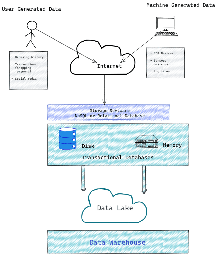
Data storage in memory is expensive and data is lost after a system restart. Memory is used to speed up access time. Disk storage is used for record-keeping and compliance purposes and for analysis. Snowflake excels at analysis of large quantities of data located on disk (or persistent storage, e.g. S3). This is also known as “Data Warehousing.” A data warehouse is often the final recipient of the data in modern IT environments. Snowflake is a database for data warehousing.
If you do not have prior experience with databases, it will help to understand what is the meaning of a data warehouse before we dive in. To understand data warehouses, let us quickly recap how database systems evolved from the 1960s. This will help understand what pain-points Snowflake solves.
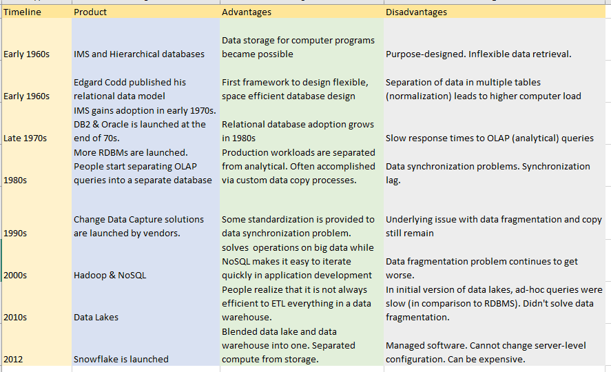
The seeds of modern databases were sown in the early 1960s by NASA & IBM during the Apollo program. To manage invoices, IBM developed a database system called IMS. This was a hierarchical database. To access data from a child element, you had to go through a parent. After learning its shortcomings, Edgar Codd from IBM proposed a relational data model in his seminal paper. This was soon followed by the world’s first relational database – System R. The viability and practicality of Codd’s model led to the foundation of relational database management systems (RDMS) such as Oracle, MySQL, and SQL Server.
What is a relational database?
In a hierarchical data model used by IMS, objects were modeled in a parent-child tree relationship. This was inflexible as data requirements changed or the system needed enhancements. For example, how will you model a student-class relationship? It is a many-to-many relationship. A student belongs to multiple classes and a class has multiple students. It is not a tree-like structure. Edgar Codd’s relational data model resolved these shortcomings. His data model provided a framework for –
- How to model entities and objects for storage in a database
- How to minimize data storage requirements
- Enable data insert, deletion, and updates
Codd’s model provided a solid foundation for the design of databases. This led to the popularity of relational databases such as Oracle and Sybase.
Let us explain Codd’s model by taking the example of student attendance. If we didn’t have two separate tables (Students table and Student Attendance table), we need to note down every student attendance as a separate record. For example,
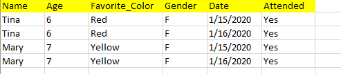
You see the problem? We are repeating student gender and age on every record. This is not necessary. Codd’s model provided a framework for reducing this redundancy. It is called the “normal form.”
Codd’s model was designed in the 1960s, well before the advent of the Internet and personal computers. While Codd’s model saves on storage requirements, it is not the compute efficient operation at the time of data retrieval. In the prior example of student attendance, if you wish to find out overall attendance by gender, you need to query two tables. This requires compute power. As the number of tables (and consequently, the number of relationships) grows, the required computing power grows as well. Despite this limitation, relational databases and SQL (the query language), have been the workhorse for more than 40 years. We can be certain that relational databases and SQL will be around in the 2030s and beyond.
What is SQL (Structured Query Language)
Going back to our student attendance example, if we wish to find out names of all female students, here is how that query will look like.
SELECT NAME FROM STUDENT WHERE GENDER='F'
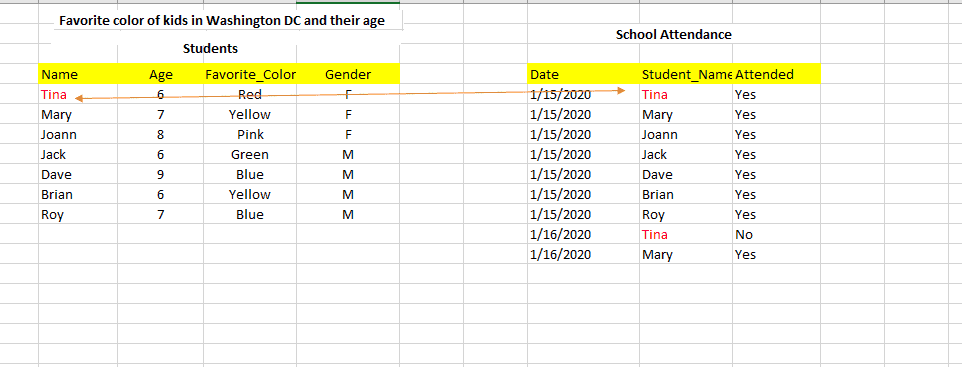
SQL can also be used to query data located in two different tables. The closest analogy is having two separate sheets in an Excel document and using operations such as LOOKUP. If we wish to find out all students who attended on ’01/15/2020′ and their favorite colors. The SQL will look as follows.
SELECT STD.NAME, STD.FAVORITE_COLOR FROM STUDENTS STD JOIN STUDENT_ATTENDANCE ATTEND ON STD.NAME = ATTEND.STUDENT_NAME WHERE ATTEND.DATE = '2020-01-15'
If you are new to SQL, you can see that our second example has more code and complexity compared to the first example. It will take more compute cycles than the first example. SQL queries can get orders of magnitude more complex than our examples.
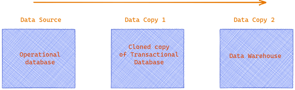
Web-scale analytical data queries (i.e. thousands of concurrent user requests on large volumes of data) require significant computing resources. Compute is a scarce resource and will remain scarce as the number of Internet-connected devices explodes higher (bitcoin mining doesn’t help either). When the CPU is busy with analytical query loads, it is not available to perform simpler transactional queries such as retrieval and insertion of single records (single transactions in our household budget example). This means that your primary production system remains unresponsive or is unavailable. This is obviously not acceptable and led to the separation of analytical and transactional workloads. This led people to cloning their production database. This cloned database was used to run complex analytical queries without impacting production databases. Data replication tools and technologies became popular with the cloning of databases. However, this was still not enough. Many companies had hundreds of database tables. Running analytical queries spanning long timestamps was very slow. Cloning of databases didn’t solve the performance problem.
What is Data Warehousing?
We saw that organizations started cloning their production databases as a solution to querying live production systems. This protected their production system. For complex systems, cloning did not resolve performance problems. What was the solution to this problem? You guessed it right. More engineering. The solution was called “Data Warehousing.”
Data Warehousing is a system used for reporting. It is built by modeling or restructuring the data from your transactional or operational system. Only the attributes and metrics of interest are brought into the warehouse. For a retailer this might mean all the sales records and the information about the products and its customers.
How is a data warehouse different from an operational database?
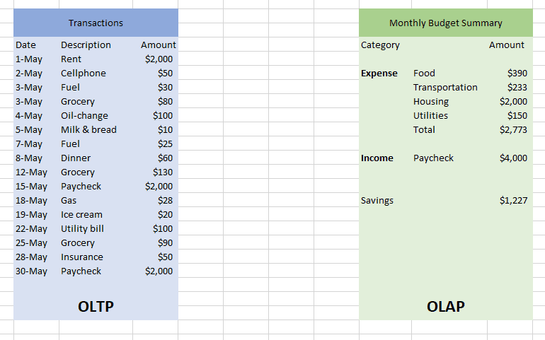
Let us take an example of a family of 3 people living in the suburbs in the United States. There are two tables below. The one on the left (blue) shows individual income and expense transactions within a month. On the right is the month-end summary. The table on the left labeled “OLTP” is your operational database. The table on the right (“OLAP”) is the output created after running analytical queries on a data warehouse.
This is a rather simple example. But imagine that you are a Walmart executive. Walmart does more than $1.5billion in sales every single day. That’s millions of transactions and individual SKUs. Producing a summary (such as the one in our household example) means aggregating millions of records. A data warehouse organizes the information from multiple tables so that creating aggregate summaries becomes quicker.
What pain-points does Snowflake solve?
Snowflake solves three business critical problems.
- Flexible compute capacity independent of storage
- Promote data reuse and sharing
- Fast analytical query performance on high-volume of data
What is flexible compute in Snowflake
Analyzing millions of records in seconds is a non-trivial computing problem. For a consistent response time to varying workloads, you need scalable and flexible compute capacity.
As your data volume grows, so does the compute time. This relationship is explained in the following diagram. As explained in the diagram, data warehousing is a performance vs cost tradeoff.
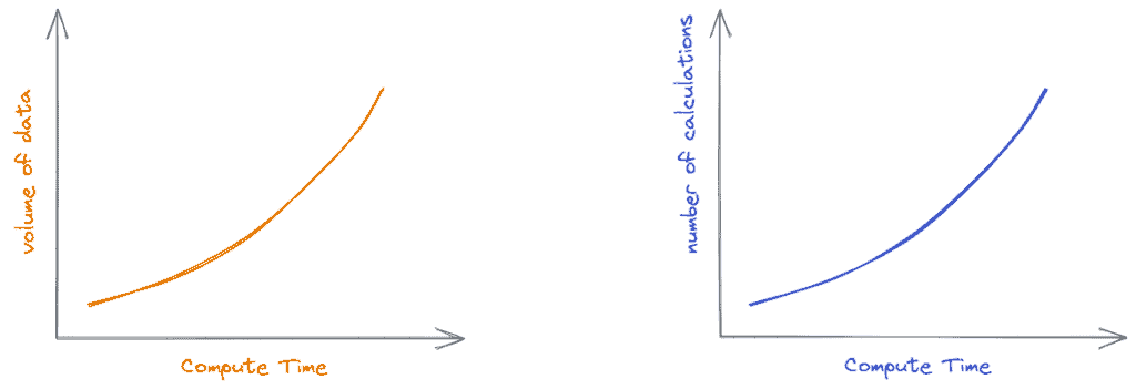
Maintaining a data warehouse is a resource-intensive (computing and human) endeavor. Resource requirements grow exponentially. Solutions to this problem involved expensive hardware until Snowflake emerged with its ability to scale compute and storage independently. Prior to Snowflake’s innovation, if you needed additional compute capacity you had to upgrade the server or add additional nodes if you were using a cluster environment.
When you create a database in Snowflake you can specify S3 (or other similar alternatives) as the storage backend. When you need additional compute capacity, you can add it or remove it when you no longer need it. The compute capacity can also be automatically scaled up or down, based on predefined thresholds.
How does Snowflake promote data reuse?
By some estimates between 60-90% of all data stored in enterprises is a copy of the original data. On the surface, data copy may appear benign. However, keeping a copy of data in-sync with its source is a non-trivial task. Besides storing data on a hard-disk, many organizations are using cloud-based storage such as S3. In the early days of the cloud, people moved the data from S3 into databases or in HDFS. As the data volume grew, this copying process became inefficient. An alternative was storing data in machine-readable binary file formats such as Parquet or Avro.
S3 is an object storage. What this means is that when you request a file, the entire file contents are retrieved. This is different from file storage which returns blocks on the disk. If your data is partitioned appropriately (e.g. by month) and your queries request data by month this can be an efficient way to store and retrieve data. This approach led to the popularity of data lakes.
Snowflake promotes data reuse by using two approaches.
- Query the data located in a data lake directly
- Promote data reuse through robust data-sharing tools
If you have large amounts of data in a data lake, Snowflake can directly query that. This saves you from having to create a copy of the data.
Another approach Snowflake uses to promote data reuse is through robust data sharing capabilities. If you wish to share data with third-parties you can efficiently do that without actually making a copy of data. The external entity needs to create a Snowflake account and they can access the data through the use of Account ID. It is also possible to share a “a slice of the data”, that is, apply the data security.
How does Snowflake achieve high performance with micro-partitions and FoundationDB?
Analytical queries, by their definition, operate on a large number of rows. Aggregation operations perform better when working on data located on the same physical node. Snowflake achieves fast performance by using a combination of:
- Micro-partitions (image below)
- A metadata database called FoundationDB
Row-based data storage keeps rows together and works great for transactional loads. Columnar stores work great for aggregation over a large number of records. Columnar engines can suffer when it comes to incremental updates and query performance is dependent on how data is distributed across multiple nodes.
Snowflake uses a hybrid approach called micro-partitions. A micro-partition is a block of data (usually 16 MB) that are kept together depending on either their insertion order or cluster key definition. Information about micro-partitions is stored in the FoundationDB. FoundationDB is a distributed key-value store. Snowflake leverages micro-partitions to do fine-grained pruning (removal of non-relevant partitions for a query). This also improves response time for update queries which is a shortcoming of many columnar stores.
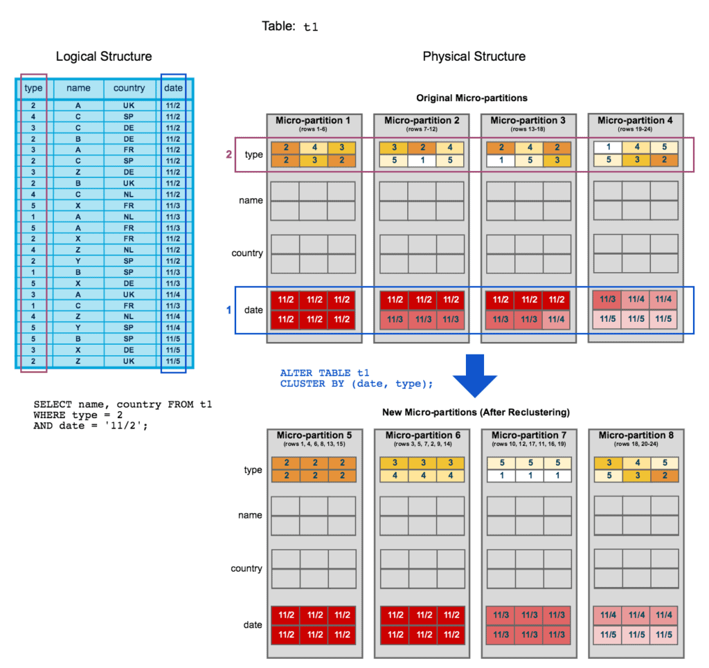
Image credit: Snowflake
In the next article on Snowflake, we will look at the market dynamics and how Snowflake could evolve into the future. If you enjoyed this article, please share it.